Lalit Pathak ¹*

1, Center of Research for Environment, Energy, and Water (CREEW), Kathmandu, Nepal

 

Manuscript link
http://dx.doi.org/10.30493/DAS.2025.520833

Abstract

High-resolution gridded population data are fundamental for disaster risk planning, emissions inventories, and urban service delivery, as they provide sub-administrative spatial detail that informs resource allocation and vulnerability assessments. In Nepal, ward-level census counts are spatially aggregated and lack the granularity required for sub-kilometer analyses, limiting their utility for fine-scale applications. This study presents an open-source QGIS workflow using the QuickOSM plugin to extract OpenStreetMap building footprints and generate a 500 m × 500 m gridded population surface for the Kathmandu Valley. Residential buildings were isolated via OSM tags, and the number of buildings within each grid cell was calculated using spatial join functions in QGIS. The population was then allocated by applying a uniform occupancy factor of 9.6 persons per building, based on existing research. Grid-level estimates were aggregated into wards and validated against Central Bureau of Statistics (CBS) 2021 census figures using Mean Absolute Error (MAE), Root Mean Squared Error (RMSE), Mean Absolute Percentage Error (MAPE), bias, Bland–Altman analysis, and Moran’s I to assess accuracy and spatial error patterns. The model estimated 3,256,317 inhabitants, 7.8% above the census total, and achieved an MAE of 3,607.5, RMSE of 4,618.8, and MAPE of 48.0%, with a positive mean error of 1,274, indicating a systematic overestimation. Bland–Altman analysis showed most ward-level differences fell within the 95% limits of agreement, while Moran’s I (Queen contiguity = 0.312, Z=8.05, p<0.001) revealed significant clustering of estimation errors in contiguous wards. This reproducible, cost-effective methodology offers a robust tool for sub-kilometer population mapping in data-scarce contexts, supporting enhanced disaster management and urban planning across Nepal and similar regions.

Keywords: QGIS, Gridded population, OpenStreetMap, Kathmandu Valley

Introduction

Gridded population data distribute population counts across a regular grid, enabling seamless integration with environmental, infrastructural, and hazard layers for informed decision‑making [1][2]. Such datasets have become fundamental to disaster risk modeling, where understanding who may be exposed to hazards like earthquakes or floods is crucial, as well as to constructing spatially explicit greenhouse gas emissions inventories and planning urban services such as water supply and healthcare [3][4].

In Nepal, the Central Bureau of Statistics (CBS) publishes detailed demographic data at the ward level; however, these figures are tied to irregular administrative boundaries and are not readily convertible to grid formats required for many spatial analyses [5]. Ward-level aggregation also masks intra-ward heterogeneity, particularly in rapidly changing urban areas like Kathmandu Valley, where population densities can vary dramatically over short distances.

Global gridded population products, such as WorldPop, LandScan, and the High-Resolution Settlement Layer (HRSL), offer alternative sources of fine-scale population estimates. WorldPop employs Random Forest dasymetric models that integrate census counts with remotely sensed and ancillary covariates to produce 100 m resolution layers [1]. At the same time, LandScan employs a multi-factorial dasymetric approach, incorporating block-level census data, transportation networks, and land cover to produce population distributions at ~90 m resolution [6]. The HRSL, developed by Meta (formerly Facebook), leverages high-resolution (0.5 m) satellite imagery and machine‑learning methods to map building footprints and settlement extents at ~30 m resolution [1].

Despite their global reach, these products face challenges in regions characterized by complex terrain and heterogeneous settlement patterns. Satellite-derived land cover may struggle to distinguish residential from non-residential structures in densely packed urban cores or dispersed rural hamlets, potentially misallocating population to uninhabited or industrial zones [4]. Moreover, rapid urban expansion between census years is common in South Asia, leading to temporal lags in official statistics.

OpenStreetMap (OSM) based approaches present a complementary pathway by harnessing a crowdsourced database of building footprints, roads, and points of interest that are continuously updated by a global mapping community. Volunteer mappers played a pivotal role in the aftermath of the 2015 Nepal earthquake, mapping over 110,000 buildings and 13,000 miles of roads within days to support relief operations [7]. The OSM building completeness shows high coverage in many urban centers, though gaps remain in informal and peri-urban areas [8].

By integrating OSM building footprints with dasymetric mapping techniques, which redistribute census counts based on ancillary spatial data, researchers can derive high-resolution, reproducible, and cost-effective gridded population surfaces. The objectives of this study are to (1) develop an open‑source QGIS workflow using the QuickOSM plugin to generate 500 m × 500 m gridded population data for Kathmandu Valley, (2) validate the resulting dataset against CBS 2021 ward-level counts to quantify accuracy, and (3) analyze spatial error patterns to identify limitations and inform future enhancements.

Materials and Methods

Study area

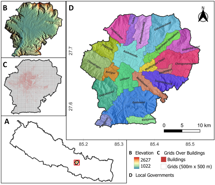
The study area is the Kathmandu valley, a core urban region in Nepal and the country’s political, economic, and cultural hub. It covers approximately 570 km², encompassing 20 local governments of the Kathmandu, Lalitpur, and Bhaktapur districts (Fig. 1). The valley is home to over 2.5 million people according to the 2021 Nepal Census [5]. It is characterized by high population density, with many multi-story buildings containing several households, presenting unique challenges for accurate population mapping. Its location in a seismically active zone further underscores the need for precise population data to support disaster risk modeling and urban planning [9].

Methods

Data acquisition and processing

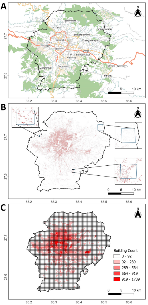
The study utilized OpenStreetMap (OSM) data to derive building footprints and estimate population distribution across Kathmandu Valley. The OSM data was downloaded using the QuickOSM [10] plugin in QGIS with a bounding extent set to the valley’s administrative boundary (Fig. 2 A).

The dataset included all building polygons (tagged as building = *). To isolate residential structures, a filter (building = residential or building = yes where residential was implied) was applied, resulting in a refined layer of residential buildings (Fig. 2 B).

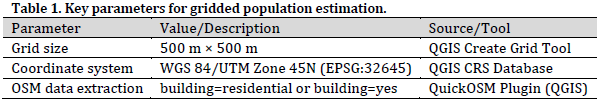
A 500 m × 500 m grid was generated using QGIS’s Create Grid tool, aligned to the WGS 84/UTM Zone 45N coordinate system (EPSG:32645) to ensure metric precision (Table 1). Building counts per grid were computed through a spatial join between the grid and the refined layer of residential buildings (Fig. 2 C).

Population per grid was estimated using the formula:

Population per grid = Building count grid × Average building family size

The average family size per residential building was assumed to be 9.6 persons, derived from a large-scale survey of 86,865 residential buildings across Kathmandu Valley [11]. Although this approach provides a robust average for the valley, it does not capture intra-ward or building-type-specific variability, which remains a limitation and an opportunity for refinement through the integration of building volume data or local micro-census data in future work. Grid-level estimates were aggregated to ward boundaries using zonal statistics to enable comparison with the 2021 census data [5].

Validation and error metrics and spatial diagnostics

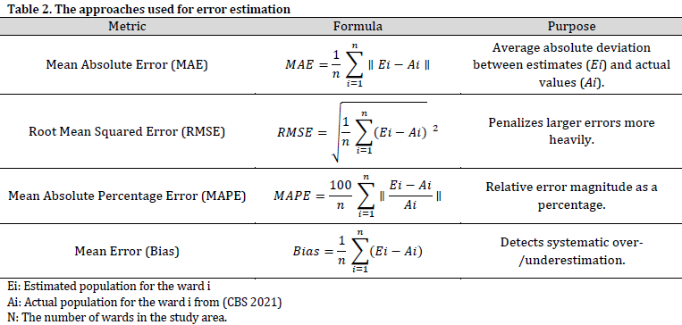
To assess model accuracy, ward-level estimated populations were compared against CBS 2021 data using the following metrics (Table 2):

Spatial patterns of estimation errors were analyzed using:

• Error Maps: Grid-level absolute errors (∣Ei​−Ai​∣) were mapped to identify localized over-/underestimation hotspots.
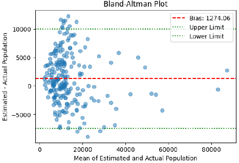
• Bland–Altman Plot: Differences (Ei​−Ai​) versus averages ((Ei​+Ai​​)/2) were plotted to visualize bias and 95% limits of agreement.
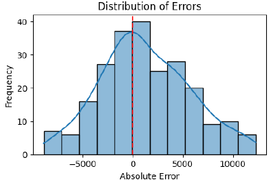
• Histogram of Absolute Errors: Frequency distribution of absolute errors to assess skewness and outlier prevalence.
• Spatial Autocorrelation: Global Moran’s I was calculated to detect clustering of errors [12]:

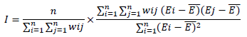
Where, wij​ is the spatial weight matrix (queen contiguity), n  is the number of grids, and Ē is the mean error. A significant positive Moran’s I (p<0.05) would indicate spatial non-randomness in errors.

Assumptions and limitations

• Uniform Family Size: The assumption of 9.6 persons per building may not reflect intra-ward variability in household density.
• OSM Data Completeness: Unmapped or misclassified buildings (e.g., informal settlements) could bias the count.
• Grid Boundary Effects: Misalignment between grids and administrative boundaries may introduce aggregation errors.

Results and Discussion

In summary, our dasymetric model allocated an estimated 3,256,317 inhabitants to 500 m × 500 m grid cells in Kathmandu Valley, overshooting the CBS 2021 total of 3,020,396 by 7.8%. The model’s global error metrics, MAE = 3,607.54, RMSE = 4,618.76, and MAPE = 48.02%, indicate relatively high error compared to advanced multi-covariate dasymetric models; yet, they are within the range reported for building count–only approaches in data-scarce contexts [13]. A consistent positive bias (Mean Error = 1,274.06) reflected a tendency to overpredict population, where building counts or assumed household sizes may misalign with reality. Spatial diagnostics reveal heterogeneous error patterns, with significant clustering of over- and underestimation across contiguous wards, underscoring the influence of local data gaps and uniform assumptions.

Global accuracy metrics

An MAE of 3607.54 persons per ward indicates the average magnitude of deviation between estimated and census counts, which, while acceptable for exploratory analyses, is high compared to refined dasymetric studies that report MAE improvements on the order of ~1–3 persons per small unit (e.g., 30 m grid cell or census block) after methodological enhancements [13]. Given that the validation in this research was performed at a much larger ward level, direct numerical comparison should be interpreted with caution. The RMSE of 4,618.76 further penalizes large deviations, suggesting that some wards exhibit substantial errors [13]. An MAPE of 48.02% falls within the “reasonable forecast” range (21–50%) as defined by Lewis (1982), while values above 51% are generally considered inaccurate; values below 10% indicate highly accurate forecasts [14][15].

Spatial distribution of population

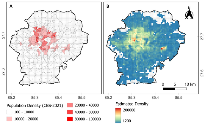
The estimated population distribution across the 500 × 500 m grids revealed significant spatial variability, with grid-level populations ranging from approximately 1,200 to over 12,800 individuals (specifically in Kathmandu and Bhaktapur districts) (Fig. 3).

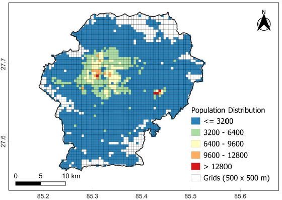
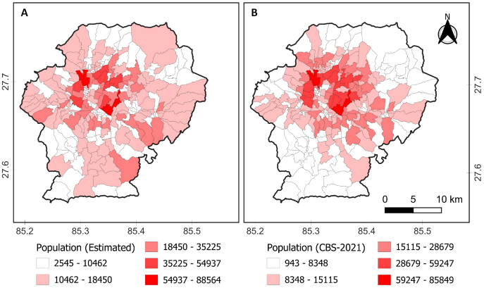
High-density clusters were predominantly located in central urban areas, while peripheral regions exhibited lower densities. When aggregated to the ward level, the estimated populations closely mirrored the spatial patterns observed in the CBS 2021 data, albeit with slight overestimations in densely populated wards (Fig. 4).

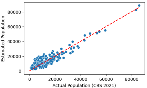
A scatter plot comparing actual versus estimated ward-level populations demonstrated a strong linear relationship, with most data points aligning closely along the line of equality, indicating a generally good fit of the model (Fig. 5). However, deviations were more pronounced in certain wards, suggesting localized discrepancies in the estimation process.

Population density comparison

The juxtaposition of census-based and grid-derived density maps (Fig. 6) highlights that, while the model reproduces major urban hotspots, it overestimates density polygons where OSM building footprints are incomplete or household sizes exceed the assumed mean. Previous fine-grained population studies have demonstrated that integrating population-sensitive POIs can reduce such biases, yielding higher accuracy than building–count–only models [16].

Error distribution and agreement analysis

The histogram of absolute errors (Fig. 7) is right-skewed, indicating that a small number of wards contribute disproportionately to the total error.

The Bland–Altman plot (Fig. 8) shows that most ward-level differences lie within the 95% limits of agreement, with a mean difference of ±1.96 × SD, confirming reasonable concordance between methods, although several outliers exceed these bounds. Importantly, Bland–Altman analysis defines the interval but does not prescribe acceptable limits; such thresholds must be set a priori based on application needs [17].

Spatial autocorrelation of errors

Global Moran’s I, computed under Queen contiguity, is 0.312 (Z=8.05, p<0.001), indicating strong positive spatial autocorrelation of estimation errors, where adjacent wards tend to share similar over‑ or underestimations (Fig. 9).

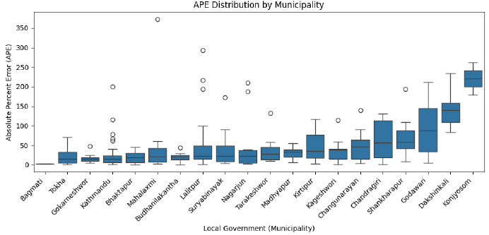
Under a K‑Nearest Neighbors (K = 1) scheme, Moran’s I falls to 0.26593 (Z=3.36, p<0.001), demonstrating that adjacency-based weights capture clustering more effectively than proximity alone. While Figure 9 displays absolute percentage errors, a closer look at signed errors reveals that peri-urban areas often exhibit overestimation, likely due to the lower actual occupancy per building than the assumed average.

Implications and future directions

The model’s systematic overestimation and significant spatial clustering of errors (Moran’s I = 0.31, p<0.001) highlight few critical limitations: (1) the assumption of a uniform household size (9.6 persons per building) inadequately captures intra-ward variability, particularly in informal settlements where household sizes may fluctuate widely; (2) uneven OpenStreetMap (OSM) coverage introduces data gaps in building counts, especially in peri-urban or rural wards, and (3) multiple households in single buildings in core urban areas. To address these challenges, future iterations should integrate ancillary covariates, such as land use classification (e.g., residential vs. commercial zones), night-time light intensity (a proxy for human activity), more accurate surveys or references for building household size, and building footprint volumes derived from high-resolution satellite imagery. For instance, studies by [18] and [3] demonstrate that night-time lights can reduce misallocations in dense urban cores by up to 30% when combined with OSM data.

Bland–Altman analysis confirmed that 95% of ward-level differences fell within the agreement limits; however, persistent outliers in informal settlements (e.g., Kathmandu’s urban periphery) underscore localized misestimates. These discrepancies mirror findings by [19], who achieved 10–20% accuracy gains by replacing uniform household sizes with building volume–adjusted occupancy rates and land use covariates. Future enhancements should prioritize using calibrated localized surveys or census microdata to reflect socioeconomic heterogeneity, implement dynamic grid sizes (e.g., 250 m in dense urban areas vs. 1 km in rural zones) to align with settlement patterns, and community mapping campaigns or convolutional neural networks (CNNs) applied to satellite imagery to fill data gaps [20][21]. Such refinements are crucial for enhancing the reliability of gridded population datasets, particularly for applications that require high spatial precision, such as disaster evacuation modeling, GHG emissions mapping, and equitable infrastructure planning. By coupling open-source geospatial data with machine learning and participatory mapping, this framework can evolve into a scalable tool for low-data regions globally.

Conclusion

This study demonstrates that an open-source QGIS workflow using OpenStreetMap building footprints can generate a 500 m × 500 m gridded population map for Kathmandu Valley, which, while moderately accurate, fills critical spatial data gaps for disaster risk management and urban planning in data-scarce regions. The model allocated 3,256,317 inhabitants, 7.8% above the CBS 2021 total, and yielded global error metrics of MAE = 3,607.54, RMSE = 4,618.76, and MAPE = 48.02%, figures comparable to other building–count–only dasymetric approaches lacking ancillary covariates. Spatial diagnostics revealed significant clustering of estimation errors, concentrated in contiguous wards, reflecting non-random biases that align with known variations in OSM data completeness across urban and peri-urban areas. Bland–Altman analysis confirmed that most ward-level differences fell within the 95% limits of agreement. Nevertheless, outliers in dense informal settlements highlight local misallocations, an issue that other studies have mitigated by integrating night-time lights to refine estimates in urban cores. Future enhancements should explore variable occupancy rates derived from local surveys, adaptive gridding techniques, and continuous OSM validation through community mapping or high-resolution imagery to enhance reliability for applications in disaster risk assessment and urban infrastructure planning.

Conflict of interest statement
The author declared no conflict of interest.
Funding statement
The author declared that no funding was received in relation to this manuscript.
Data availability statement
The author declared that all used data and data sources are mentioned in the manuscript. All datasets will be available upon reasonable request from the corresponding author.

References

1. Tatem AJ. WorldPop, open data for spatial demography. Sci. data. 2017;4(1):1-4. DOI
2. Leyk S, Gaughan AE, Adamo SB, De Sherbinin A, Balk D, Freire S, Rose A, Stevens FR, Blankespoor B, Frye C, Comenetz J. The spatial allocation of population: a review of large-scale gridded population data products and their fitness for use. Earth Syst. Sci. Data. 2019;11(3):1385-409. DOI
3. Zhuang H, Liu X, Li B, Wu C, Yan Y, Zeng L, Zheng C. Mapping high-resolution global gridded population distribution from 1870 to 2100. Sci. Total Environ. 2024;955:176867. DOI
4. Stevens FR, Gaughan AE, Linard C, Tatem AJ. Disaggregating census data for population mapping using random forests with remotely-sensed and ancillary data. PloS one. 2015;10(2):e0107042. DOI
5. National Statistics Office: Kathmandu. CBS National Population and Housing Census 2021. Government of Nepal, Nepal. 2021.
6. Rose AN, Bright E. The LandScan Global Population Distribution Project: current state of the art and prospective innovation. Oak Ridge National Laboratory. 2014.
7. Sneed, A. The Open Source Maps That Made Rescues in Nepal Possible. WIRED. 2015.
8. Zhou Q, Zhang Y, Chang K, Brovelli MA. Assessing OSM building completeness for almost 13,000 cities globally. Int. J. Digit. Earth. 2022;15(1):2400-21. DOI
9. Carpenter S, Grünewald F. Disaster preparedness in a complex urban system: the case of Kathmandu Valley, Nepal. Disasters. 2016;40(3):411-31. DOI
10. Trimaille, E. QuickOSM. Version 2.4.1 [Software]. 2025.
11. Thapa AK, Thapa BK. Analyzing Willingness to Pay for Improved Tap Water Quality: A Case of Kathmandu Valley of Nepal. Econ. J. Dev. Issues. 2020. DOI
12. Fortin MJ, Drapeau P, Legendre P. Spatial autocorrelation and sampling design in plant ecology. Progress in theoretical vegetation science. 1990;209–22. DOI
13. Baynes J, Neale A, Hultgren T. Improving intelligent dasymetric mapping population density estimates at 30 m resolution for the conterminous United States by excluding uninhabited areas. Earth Syst. Sci. Data. 2022;14(6):2833-49. DOI
14. Lewis CD. Industrial and business forecasting methods: A practical guide to exponential smoothing and curve fitting. Butterworth Scientific: London; Boston. 1982.
15. Kasemset C, Sae-Haew N, Sopadang A. Multiple regression model for forecasting quantity of supply of off-season longan. Chiang Mai Univ. J. Nat. Sci. 2014;13(3):391-402. DOI
16. Zhao Y, Li Q, Zhang Y, Du X. Improving the accuracy of fine-grained population mapping using population-sensitive POIs. Remote Sens. 2019;11(21):2502. DOI
17. Giavarina D. Understanding bland altman analysis. Biochem. Med. 2015;25(2):141-51. DOI
18. Wang L, Fan H, Wang Y. Improving population mapping using Luojia 1-01 nighttime light image and location-based social media data. Sci. Total Environ. 2020;730:139148. DOI
19. Wu B, Yang C, Wu Q, Wang C, Wu J, Yu B. A building volume adjusted nighttime light index for characterizing the relationship between urban population and nighttime light intensity. Comput. Environ. Urban. Syst. 2023;99:101911. DOI
20. McKeen T, Bondarenko M, Kerr D, Esch T, Marconcini M, Palacios-Lopez D, Zeidler J, Valle RC, Juran S, Tatem AJ, Sorichetta A. High-resolution gridded population datasets for Latin America and the Caribbean using official statistics. Sci. Data. 2023;10(1):436. DOI
21. Stathakis D, Baltas P. Seasonal population estimates based on night-time lights. Comput. Environ. Urban. Syst. 2018;68:133-41. DOI

Cite this article:

Pathak,L. A QGIS-based approach of developing gridded population data for the Kathmandu Valley using OpenStreetMap building data. DYSONA – Applied Science, 2026;7(1): 50-60. doi: 10.30493/das.2025.520833